Firstly, we need to think about why we need to reduce the dimensionality of a feature set. You will find that when we get a large size of data, the speed of calculation is extremely slow. Between these features, we can find some set are unrelated and some are highly related. Some people may ask is there a solution to quick the speed but don’t sacrifice the accuracy? So I concluded three reasons to do dimensionality reduction:

1. Remove features that have no correlation with the target distribution
2. Remove/combine features that have redundant correlation with target distribution
3. Extract new features with a more direct correlation
   with target distribution

In this article, I am going to talk about method, Correlation Based Feature Selection and Principal Component Analysis. Some Matlab code will be used to illustrate it.

Correlation Based Feature

Correlation based feature selection (CFS) selects features in a forward-selection manner. And it is a iterative procedure, below are the steps it should take:

1. Start with an empty set of selected features S_k, and a full set of initial features F, initialise k=1
2. For each feature f in F, calculate the Pearson’s product-moment correlation r_cf between f and the target value t
3. For each feature f in F, calculate the sum of correlations between f and all the features already in S_k
4. Select the feature that maximises CF
   S for this iteration, add it to S_k and remove it from F. Set k = k+1
5. Repeat steps 2-4 until the CFS value starts to drop (convergence)
   And the main function of CFS is
   
   To illustrate this formula and the procedure b

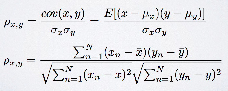
etter way, we need to know how to calculate the correlations. Here we calculate the Pearson’s (product-moment) correlation. This value is between -1 and 1 with 1being fully correlated, -1 being negatively correlated, and 0 no correlation. The formula should be:

And the Matlab code for calculating it should be:

1
2
3
4
5
6
7
8
9
10
11
12
13
14
15
16
17
18
19
20
21

function [ co ] = pearson_product_moment_correlation( feature, target )
    avg_x = sum(feature)/size(feature, 1);
    avg_y = sum(target)/size(target, 1);
    co_a = 0;
    for i=1:size(feature, 1)
        co_a = co_a+(feature(i,1)-avg_x)*(target(i,1)-avg_y);
    end
    co_b = 0;
    for i=1:size(feature, 1)
        co_b = co_b+(feature(i,1)-avg_x)*(feature(i,1)-avg_x);
    end
    co_b = sqrt(co_b);
    co_c = 0;
    for i=1:size(target, 1)
        co_c = co_c+(target(i,1)-avg_y)*(target(i,1)-avg_y);
    end
    co_c = sqrt(co_c);
    co = co_a/(co_b*co_c);
end

Then each time when adding a new feature to S_k do this calculation and select the maximum CFS for each iteration. When the CFS value decreases, stop the iteration.

Principal Component Analysis

Luckily, Matlab has a PCA function for us to do the calculation. However, we need to truly understand what PCA is. PCA requires calculation of:

1. mean of observed variables
2. covariance of observed variables
3. eigenvalue/eigenvector computation of covariance matrix

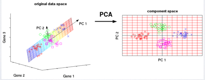
In Wikipedia, PCA is defined as Principal component analysis (PCA) is a statistical procedure that uses an orthogonal transformation to convert a set of observations of possibly correlated variables into a set of values of linearly uncorrelated variables called principal components. If let me explain it, I will say that it emphasizes variation between features and bring out strong patterns in a dataset. Now, you have the brief introduction of what PCA is. then take a look at PCA function in Matlab. To be specific, pca returns as first variable [coeff] the principal components (PCs), ordered by descending eigenvalues (i.e. accounting for increasingly less variance in the data). The second variable [score] returns the actual eigenvalues, while the third variable [latent] returns the relative variance accounted for by each PC.

There is a Matlab example code for PCA:

1
2
3
4
5

data = load('your_data.mat');
[coeff, score, latent] = pca(data.x);
x = score(:, 1);
y = score(:, 2);
scatter(x, y, 25, data.y, 'filled');

In this demo, I just select two features to draw a 2D scatter figure. You can select more, and it depends on your circumstance. Hope you all have understand that. 🙂 If you have any questions, please comment below. 🙂 Willing to discuss with you. 🙂

Comments: